A simple introduction to probability, expected value, and the law of large numbers, with intuitive examples and an explanation of random walks in financial markets.
We were discussing “dad” jokes at work when a colleague shared a classic probability line: “A student who didn’t study for his probability test was asked how he felt. He replied, ‘I’ll take my chances.’”
This joke perhaps reflects how many of us feel about probability. We tend to have an intuitive sense of what it is but often struggle to explain it clearly.
In this post, I aim to provide a simple introduction to key probability concepts and how they are applied to what are known as “random walks”. This serves as a primer for more advanced topics.
The Law of Large Numbers
One of the fundamental theorems in probability is the Law of Large Numbers. It states that, as the number of independent trials increases, the frequency of obtaining an outcome converges to its true probability.
This can be illustrated using a six-sided die. If we roll a die only a small number of times, the results may appear biased towards a particular number. For example, we might observe several 6s and very few of the other numbers. However, as the number of independent rolls increases, the relative frequencies begin to stabilise.
For a fair die, each number has a probability of 1/6, so over a large number of rolls, approximately one-sixth of the outcomes will be 6s, one-sixth will be 5s, and so on.
In this way, results from a small number of trials can appear random and unbalanced, whereas a large number of trials reveals the underlying structure of the probability distribution.
Expected Value
The Law of Large Numbers leads naturally to the concept of expected value. This idea was first introduced into probability theory by the Dutch polymath Christiaan Huygens.
To build intuition, we begin with an informal definition before introducing a more formal one. The expected value can be thought of as the long-run average outcome you would expect if a random process were repeated many times.
Let us continue with the die example. Since each outcome has an equal probability of 1/6, the expected value is calculated as the sum of each possible outcome multiplied by its corresponding probability:
(1/6 × 1) + (1/6 × 2) + (1/6 × 3) + (1/6 × 4) + (1/6 × 5) + (1/6 × 6) = 3.5
The expected value of this experiment is therefore 3.5. This does not mean we will ever roll a 3.5; rather, it means that the average of many rolls will tend towards 3.5.
For those that like formal mathematical definitions, if we assume that X is a random variable with a discrete probability distribution pj=P(X=xj) for j = 1 , . . . , M, then the expected value defined by E(x) is:

The Drunkard’s Walk
Having introduced the Law of Large Numbers and expected value, we can now consider the concept of a random walk.
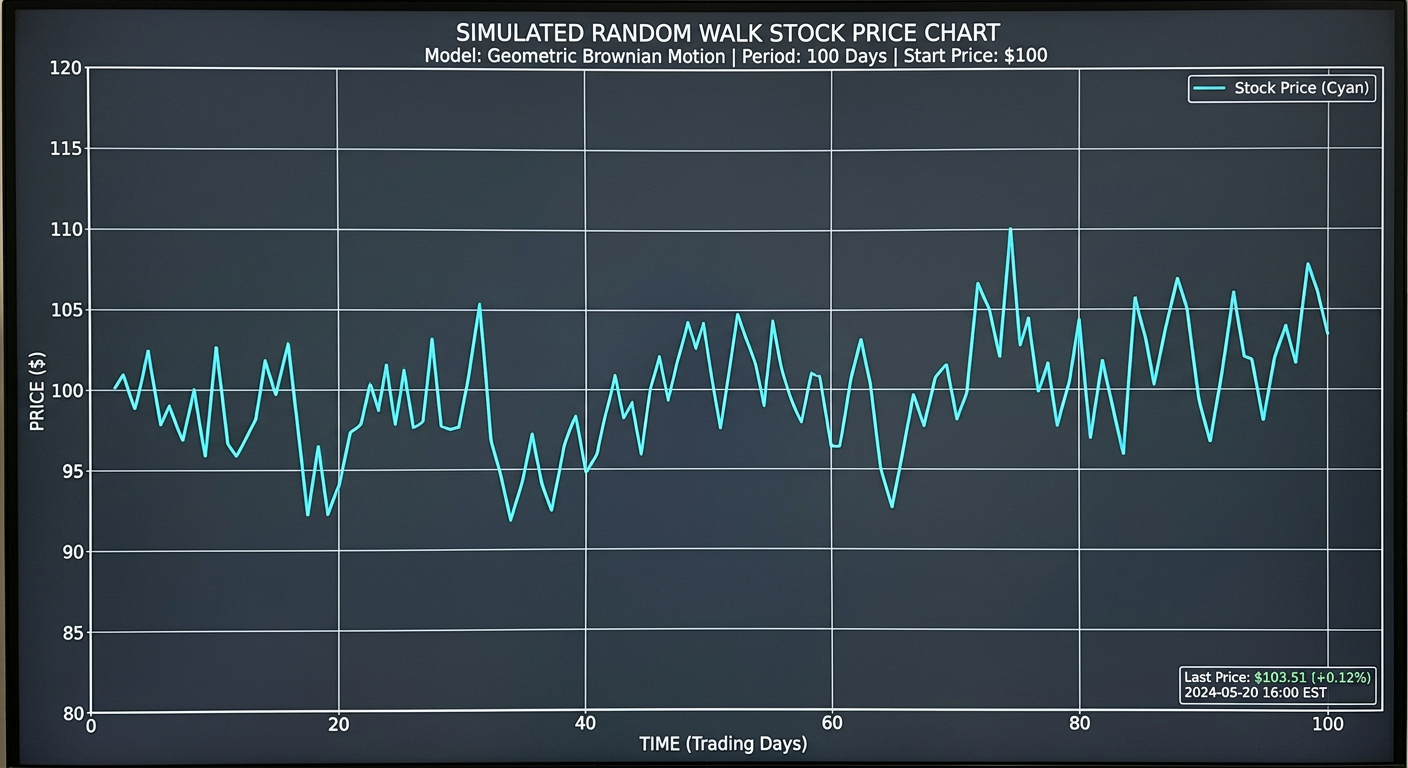
A random walk is often illustrated through the example of the “drunkard’s walk”. Imagine a person leaving a pub late at night and attempting to walk home in a straight line. With each step, they randomly move one step to the left or one step to the right, each with probability 1/2.
Because each step is random and independent, the overall path becomes irregular and difficult to predict, much like the short-term movement of financial markets.
Applying the concept of expected value to this random walk, we find that the expected change in position at each step is 0. In other words, there is no overall tendency to move in one direction or the other. Put another way, the best estimate of the drunkard’s future position is simply their current location.
This idea is central in financial mathematics. Such processes are often modelled as martingales, where the best estimate of a future value is its current value.
This modelling approach is linked to the assumption that markets are free of arbitrage. Under this assumption, the discounted price of tradable assets behaves like a martingale under a suitable probability measure. More on martingales in future posts.
Closing Remarks
These simple ideas, probability distributions, expected value, and random walks, form the foundation of many models used in finance. While real markets are more complex than this basic framework, these concepts provide a useful starting point for understanding how uncertainty is modelled mathematically.
In future posts, we will build on these ideas to explore martingales, stochastic processes, and their applications in financial modelling.
If you’ve enjoyed reading,
you can support the site with a coffee, helps keep the walks going. buymeacoffee.com/walkcuriously